Code walk through
Load in the usual packages, and ggthemes so I can use the fivethirtyeight ggplot2 theme.
library(tidyverse)
library(lubridate)
library(ggthemes)

board_games <- read_csv("https://raw.githubusercontent.com/rfordatascience/tidytuesday/master/data/2019/2019-03-12/board_games.csv")
Let’s get a look at the data.
glimpse(board_games)
## Observations: 10,532
## Variables: 22
## $ game_id        <dbl> 1, 2, 3, 4, 5, 6, 7, 8, 9, 10, 11, 12, 13, 14, ...
## $ description    <chr> "Die Macher is a game about seven sequential po...
## $ image          <chr> "//cf.geekdo-images.com/images/pic159509.jpg", ...
## $ max_players    <dbl> 5, 4, 4, 4, 6, 6, 2, 5, 4, 6, 7, 5, 4, 4, 6, 4,...
## $ max_playtime   <dbl> 240, 30, 60, 60, 90, 240, 20, 120, 90, 60, 45, ...
## $ min_age        <dbl> 14, 12, 10, 12, 12, 12, 8, 12, 13, 10, 13, 12, ...
## $ min_players    <dbl> 3, 3, 2, 2, 3, 2, 2, 2, 2, 2, 2, 2, 3, 3, 2, 3,...
## $ min_playtime   <dbl> 240, 30, 30, 60, 90, 240, 20, 120, 90, 60, 45, ...
## $ name           <chr> "Die Macher", "Dragonmaster", "Samurai", "Tal d...
## $ playing_time   <dbl> 240, 30, 60, 60, 90, 240, 20, 120, 90, 60, 45, ...
## $ thumbnail      <chr> "//cf.geekdo-images.com/images/pic159509_t.jpg"...
## $ year_published <dbl> 1986, 1981, 1998, 1992, 1964, 1989, 1978, 1993,...
## $ artist         <chr> "Marcus Gschwendtner", "Bob Pepper", "Franz Voh...
## $ category       <chr> "Economic,Negotiation,Political", "Card Game,Fa...
## $ compilation    <chr> NA, NA, NA, NA, NA, NA, NA, NA, NA, NA, NA, NA,...
## $ designer       <chr> "Karl-Heinz Schmiel", "G. W. \"Jerry\" D'Arcey"...
## $ expansion      <chr> NA, NA, NA, NA, NA, NA, NA, NA, NA, "Elfengold,...
## $ family         <chr> "Country: Germany,Valley Games Classic Line", "...
## $ mechanic       <chr> "Area Control / Area Influence,Auction/Bidding,...
## $ publisher      <chr> "Hans im Glück Verlags-GmbH,Moskito Spiele,Vall...
## $ average_rating <dbl> 7.66508, 6.60815, 7.44119, 6.60675, 7.35830, 6....
## $ users_rated    <dbl> 4498, 478, 12019, 314, 15195, 73, 2751, 186, 12...
First off, I want to see the cumulative board game total count over the years.
cumulative <-
  board_games %>%
  count(year_published) %>%
  mutate(cumulative = cumsum(n))

cumulative
## # A tibble: 67 x 3
##    year_published     n cumulative
##             <dbl> <int>      <int>
##  1           1950     4          4
##  2           1951     2          6
##  3           1952     3          9
##  4           1953     3         12
##  5           1954     3         15
##  6           1955     4         19
##  7           1956     6         25
##  8           1957     2         27
##  9           1958     8         35
## 10           1959     7         42
## # ... with 57 more rows
cumulative %>%
  ggplot(aes(year_published, cumulative)) +
  geom_point() +
  geom_line() +
  scale_x_continuous(breaks = seq(1950, 2020, 10)) +
  scale_y_continuous(labels = scales::comma) +
  labs(x = "Year",
       y = "Cumulative No. of Board Games") +
  theme_fivethirtyeight()
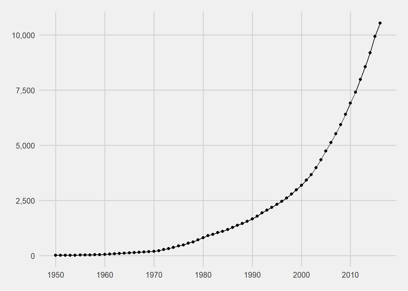
The number of board games picked up in the 70s and really got going exponential after 2000.
I want to do the same thing, but look at how the use of different game mechanics has changed over the years. A game mechanic is how a game is played like rolling dice, drawing, or storytelling. Let’s take a look at the mechanic column.
board_games %>% select(mechanic)
## # A tibble: 10,532 x 1
##    mechanic
##    <chr>
##  1 Area Control / Area Influence,Auction/Bidding,Dice Rolling,Hand Managem~
##  2 Trick-taking
##  3 Area Control / Area Influence,Hand Management,Set Collection,Tile Place~
##  4 Action Point Allowance System,Area Control / Area Influence,Auction/Bid~
##  5 Hand Management,Stock Holding,Tile Placement
##  6 Dice Rolling
##  7 Area Enclosure,Pattern Building,Pattern Recognition,Tile Placement
##  8 Modular Board
##  9 Area Control / Area Influence,Tile Placement
## 10 Card Drafting,Hand Management,Point to Point Movement,Route/Network Bui~
## # ... with 10,522 more rows
It looks like a board game can have multiple mechanic categories as we see here separated by commas. What I need to do to analyze this type of data is force each row to have just one category while maintaining some contextual information. In this case I just want to keep a hold of the year column. Before we start, I’m just curious, what game had the most combinations of game mechanics?
board_games %>%
  select(year_published, name, mechanic) %>%
  mutate(m_count = str_count(mechanic, ",")) %>%
  arrange(desc(m_count))
## # A tibble: 10,532 x 4
##    year_published name            mechanic                          m_count
##             <dbl> <chr>           <chr>                               <int>
##  1           2015 504             Area Control / Area Influence,Ar~      17
##  2           2014 Emperor's New ~ Acting,Action Point Allowance Sy~      14
##  3           2013 Patchistory     Action Point Allowance System,Ar~      11
##  4           2013 City of Remnan~ Action Point Allowance System,Ar~      10
##  5           2016 Pyramid Arcade  Area Control / Area Influence,Be~      10
##  6           2011 Mage Knight Bo~ Card Drafting,Co-operative Play,~       9
##  7           2012 Exodus: Proxim~ Area Control / Area Influence,Ar~       9
##  8           2015 Chaosmos        Action Point Allowance System,Ca~       9
##  9           2014 Sons of Anarch~ Action Point Allowance System,Ar~       9
## 10           1985 Advanced Squad~ Auction/Bidding,Dice Rolling,Hex~       8
## # ... with 10,522 more rows
Hmm, 504, I’m not familiar with it. Looks like settlers of catan after with a cash system after looking here. Probably very complicated.
Now on to the data manipulation. I’ll use tidyr::separate_rows() to separate the categories and puts each of them into their own row.
mechanics_count <-
  board_games %>%
  select(year_published, mechanic) %>%
  drop_na(mechanic) %>%
  separate_rows(mechanic, sep = ",")

mechanics_count
## # A tibble: 23,950 x 2
##    year_published mechanic
##             <dbl> <chr>
##  1           1986 Area Control / Area Influence
##  2           1986 Auction/Bidding
##  3           1986 Dice Rolling
##  4           1986 Hand Management
##  5           1986 Simultaneous Action Selection
##  6           1981 Trick-taking
##  7           1998 Area Control / Area Influence
##  8           1998 Hand Management
##  9           1998 Set Collection
## 10           1998 Tile Placement
## # ... with 23,940 more rows
Now we have all the game mechanics used with their corresponding year. Notice we went from 9.5K rows to 23.9K which is expected.
mechanics_count %>%
  select(mechanic) %>%
  unique() %>%
  drop_na(mechanic) %>%
  nrow()
## [1] 51
Before we get into plotting, I need to find the top 6 most occurring game mechanics. Having a total of 51 different game mechanics would make my plot hard to understand so let’s keep it simple.
top_mechanics <-
  mechanics_count %>%
  count(mechanic, sort = T) %>%
  top_n(n = 6, wt = n) %>%
  pull(mechanic)

top_mechanics
## [1] "Dice Rolling"           "Hand Management"
## [3] "Set Collection"         "Hex-and-Counter"
## [5] "Variable Player Powers" "Tile Placement"
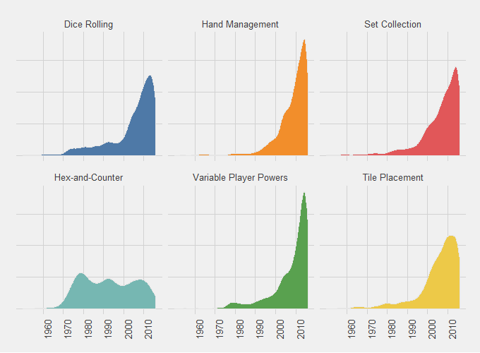
Perfect, now lets plot them using a faceted density plot.
mechanics_count %>%
  filter(mechanic %in% top_mechanics) %>%
  mutate(mechanic = factor(mechanic, levels = top_mechanics)) %>%
  ggplot(aes(year_published, fill = mechanic)) +
  geom_density(col = "grey90", show.legend = F) +
  facet_wrap(~mechanic, ncol = 3) +
  scale_x_continuous(breaks = seq(1960, 2010, 10)) +
  scale_fill_tableau() +
  labs(title = "Most Occurring Board Game Mechanics over the years") +
  theme_fivethirtyeight() +
  theme(axis.text.y = element_blank(),
        axis.text.x = element_text(angle = 90))
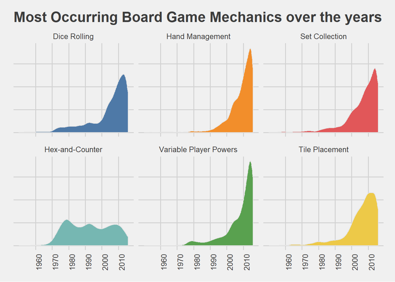
All but one game mechanic seem to have rising in popularity rather quickly over the past two decades, while the Hex-and-Counter method has maintained a good share for for almost 40 years!