scrips <- read_csv("lds-scriptures.csv")
names <- read_rds(gzcon(url("https://byuistats.github.io/M335/data/BoM_SaviorNames.rds")))
verse <- read_lines("https://byuistats.github.io/M335/data/2nephi2516.txt")

Background

In 1978, Susan Easton Black calculated the average number of verses per mention of Christ’s name by each book in the Book of Mormon. She found that Christ’s name is mentioned about every 1.7 verses. But what is the average number of words between each reference of Christ outside the context of books, chapters, and verses?

Data Analysis

names <- names %>% arrange(desc(nchar)) 
#------- This prevents splitting inside of larger references
names2 <- names$name 
#-------------------------- From tibble to list
names3 <- str_c(names2, collapse = "|") 
#------- Creates one string w/ all references seperated by or statements

BoM <- scrips %>% 
  filter(volume_id == 3) %>% #------------------ Filter for just Book of Mormon
  select(scripture_text) %>% #------------------ We just want scripture text
  str_c(collapse = " ") %>%  #------------------ Creates one string of whole Book of Mormon
  str_split(names3) #--------------------------- Splits the string into many based on references
  #map(function(x) str_count(x, "\\w"))

for (split in BoM) { #-------------------------- Lets iterate over all those new strings
    count <- str_count(split, "\\w+") #--------- Counts the words in each string, assigns to count
  }

count_tbl <- tibble(y = count, #---------------- Turn vector into tibble
                    x = seq_along(y)) %>% #----- Create index variable
  filter(x != 1, x != 4071) #------------------- Trim off frist and last observation since they aren't words between a reference

ggplot(count_tbl,aes(x = y)) +
  geom_histogram(bins = 150, 
                 fill = "#969696", 
                 col = "white") +
  geom_vline(xintercept = count_tbl %>% {mean(.$y)}, 
             col = "red", 
             size = 1) +
  annotate(geom = "text",
           x = count_tbl %>% {mean(.$y)} + 40,
           y = 1000,
           label = paste("Mean = ", count_tbl %>% {round(mean(.$y),2)})) +
  scale_x_continuous(breaks = seq(0,500,50)) +
  coord_cartesian(xlim = c(0,500)) +
  labs(x = "References",
       y = "Occurances",
       title = "Distribution of Words Between References of Christ") +
  theme_pander()

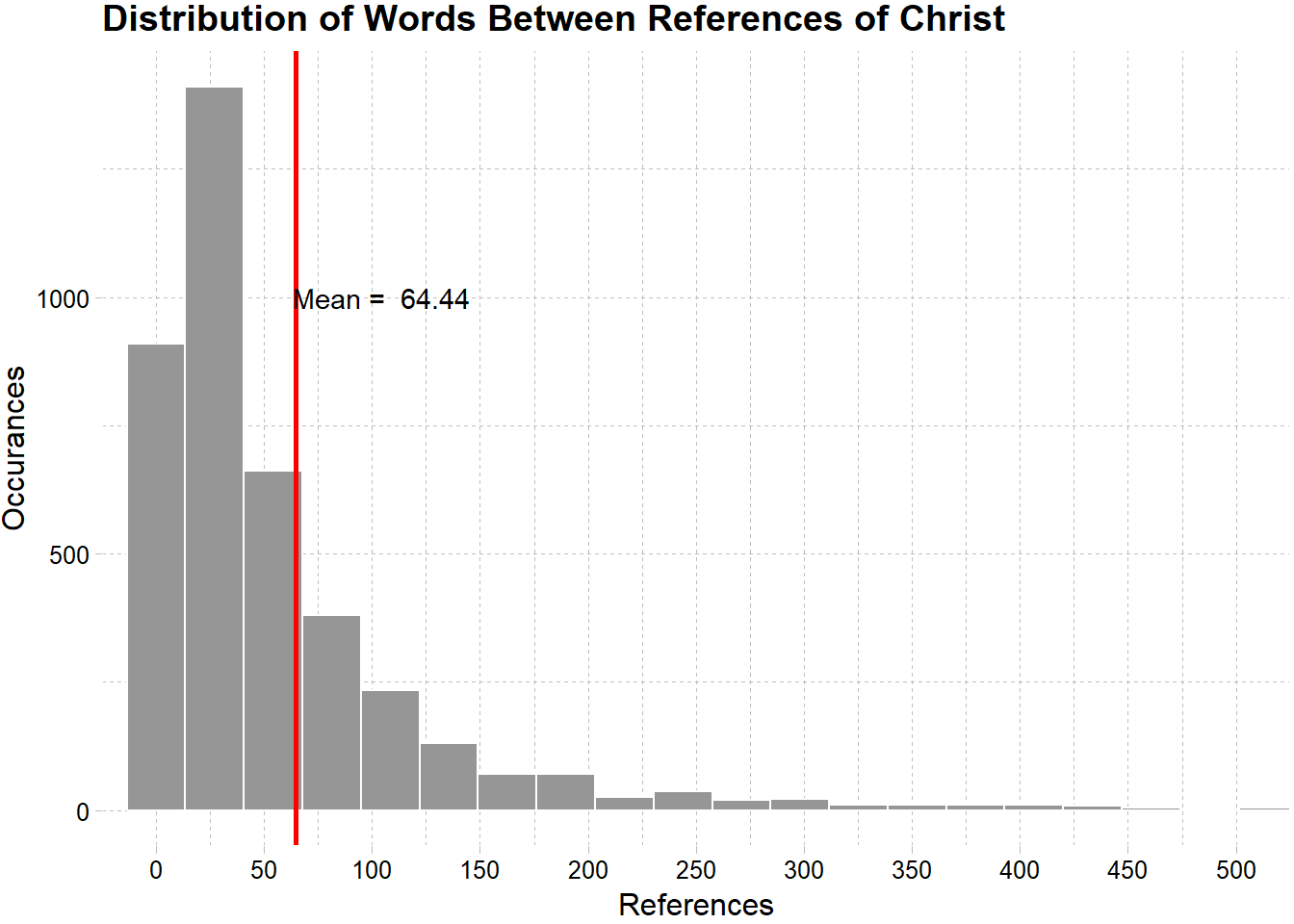
The answer to the original question is 64.44. Or at least around that number. But with the data we have, there is so much more we can do with it.

ggplot(count_tbl,aes(x = x, y = y)) +
  geom_point(color = "#08519c",
             alpha = .2) +
  geom_smooth(color = "#FADA23") +
  scale_x_continuous(labels = scales::comma) +
  scale_y_continuous(labels = scales::comma) +
  labs(title = "Some Word Counts Between References are Very Large",
    x = "References",
    y = "Word Count") +
  theme_pander()

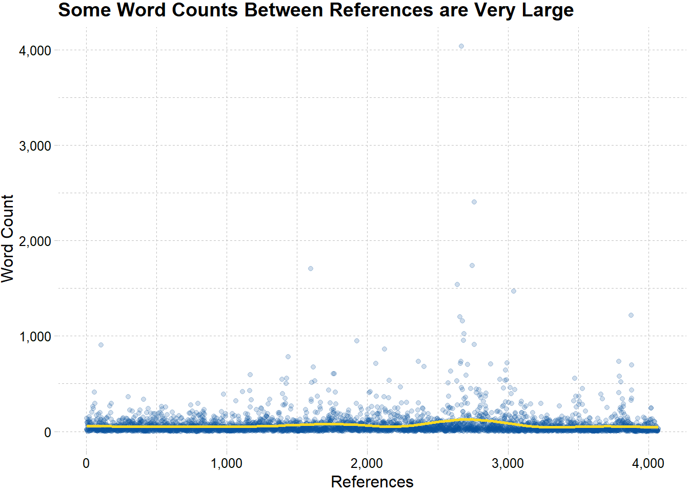
It looks like there are a few times where the word count is large between a reference of Christ. The next plot zooms in on the data to make more sense of it.

ggplot(count_tbl,aes(x = x, y = y)) +
  geom_point(color = "#08519c",
             alpha = .2) +
  geom_smooth(color = "#FADA23",
              se = F,
              size = 2) +
  coord_cartesian(ylim = c(0,400)) +
  scale_x_continuous(labels = scales::comma) +
  scale_y_continuous(labels = scales::comma) +
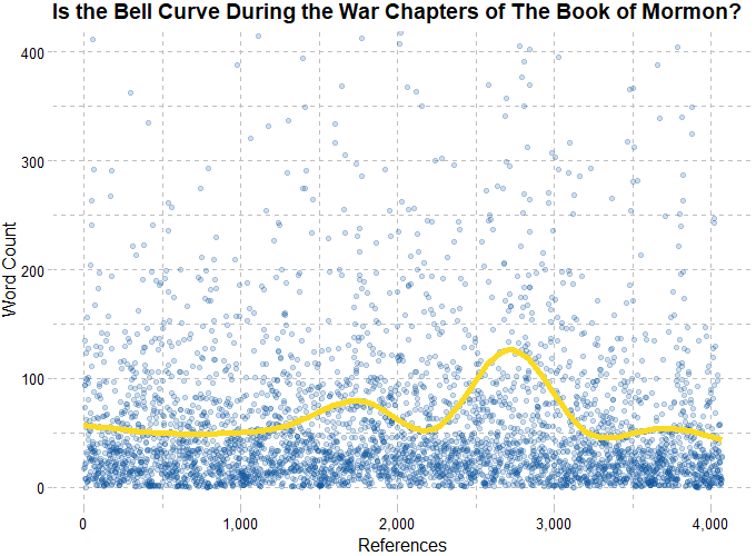
  labs(title = "Is the Bell Curve During the War Chapters of The Book of Mormon?",
    x = "References",
    y = "Word Count") +
  theme_pander()

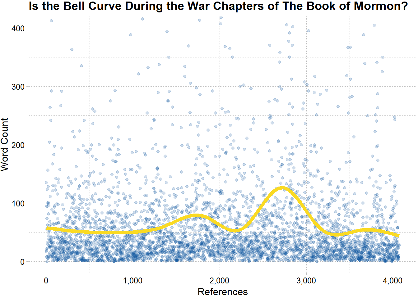
We can interpret this plot as the lower the yellow line, the more Christ is referred to in the book of Mormon. It looks like there are two periods in the Book of Mormon where Christ was referred to a little less. Could this be the war chapters? Since I used a for loop to obtain the word count, I lost the contextual information like book and chapter titles. The following code preserves this information with the help of nesting and un-nesting data in a data frame.

books <- c("1 Nephi","2 Nephi","Jacob","Enos",
           "Jarom","Omni","Words of Mormon",
           "Mosiah","Alma","Helaman","3 Nephi",
           "4 Nephi","Mormon","Ether","Moroni")

cnt_byverse <- scrips %>% 
  filter(volume_id == 3) %>% 
  # Filter for just Book of Mormon
  select(book_title, verse_title, 
         scripture_text) %>% 
  # Select scripture text with book and verse title
  mutate(nested = str_split(scripture_text, names3), 
         # Split each verse by reference in each verse
         not_split = case_when(
           str_detect(nested, "c\\(") ~ FALSE,
           !str_detect(nested, "c\\(") ~ TRUE)) %>%
  # T if verse was split. F if no reference and no split
  unnest() %>%
  # Since splitting the verses created a nested column, this will unnest that column and expand the rows accordingly
  mutate(btw_length = str_count(nested, "\\w+"), 
         # Counts the words in each seperation or verse
         index = seq_along(btw_length), 
         # Add index variable
         book_title = factor(book_title, levels = books) %>% fct_rev()) 
# Reversing the levels makes them appear in the correct order once I plot the data

Now we know which book each instance of words between references belong. We can use this to plot the same information below. You will notice that the line seems to be flatter than before. This is because the method I used also considers verses with no references as an instance to derive a word count from. Although this provides data that wouldn’t be used to answer the original question, we can still see the two periods where references occurred less.

split_book <- cnt_byverse %>% 
  group_by(book_title) %>% 
  summarise(min = min(index))

ggplot(cnt_byverse, aes(index, btw_length)) +
  geom_point(aes(color = book_title),
             alpha = .2,
             show.legend = F) +
  geom_smooth(color = "#FADA23",
              se = F,
              size = 2) +
  scale_color_cyclical(values = c("#CCCCCC", "#7F7F7F")) +
  geom_vline(xintercept = split_book$min, col = "#08519c",
             linetype = "dotted", size = 1) +
  annotate(geom = "text", x = c(7050,7300), y = 100, 
           label = c("Alma", "Helaman"), angle = 90) +
  labs(title = "Word Count Is Largest End of Alma Beginning of Helaman",
    x = "References, By Book",
    y = "Word Count") +
  theme_pander()

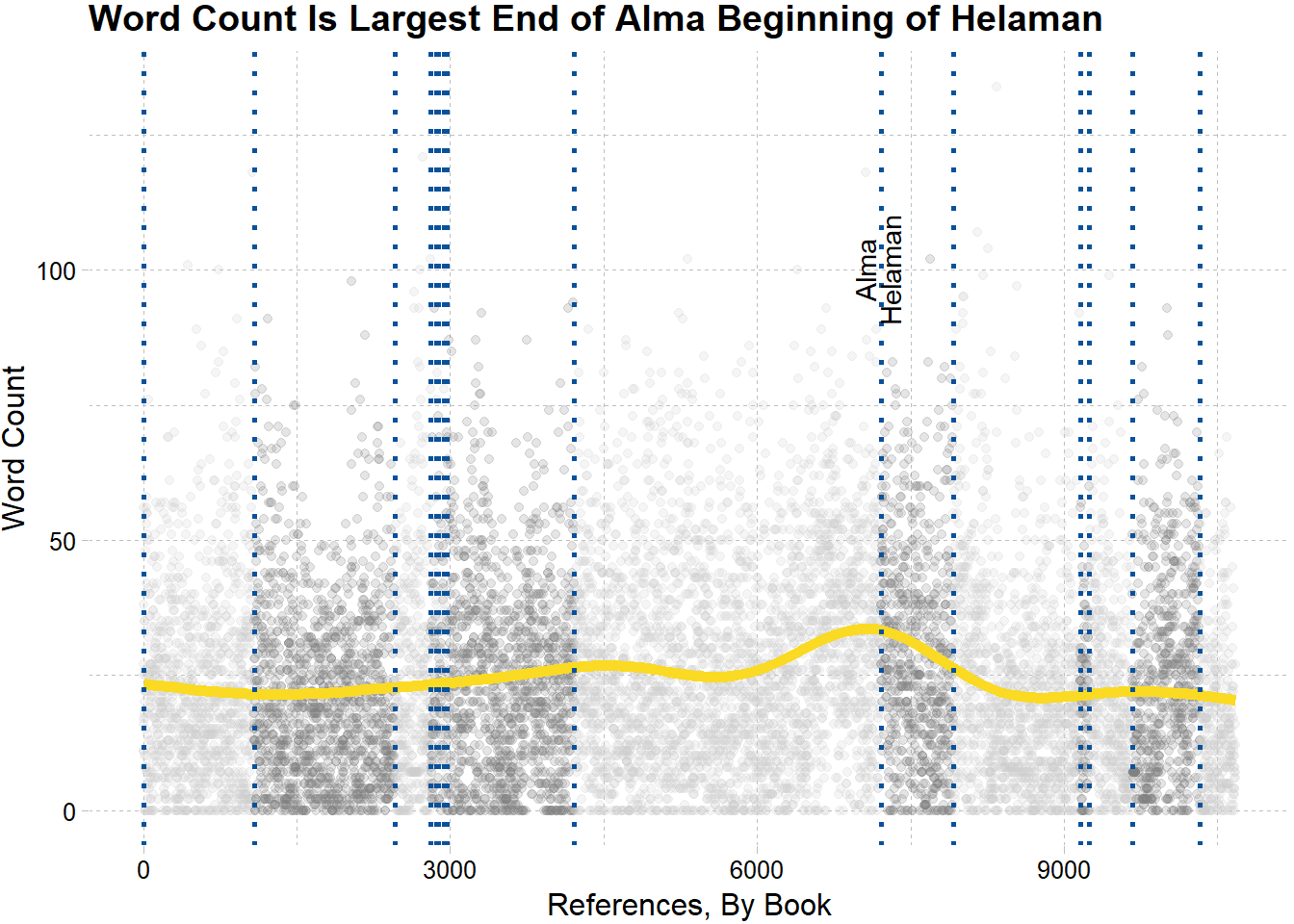
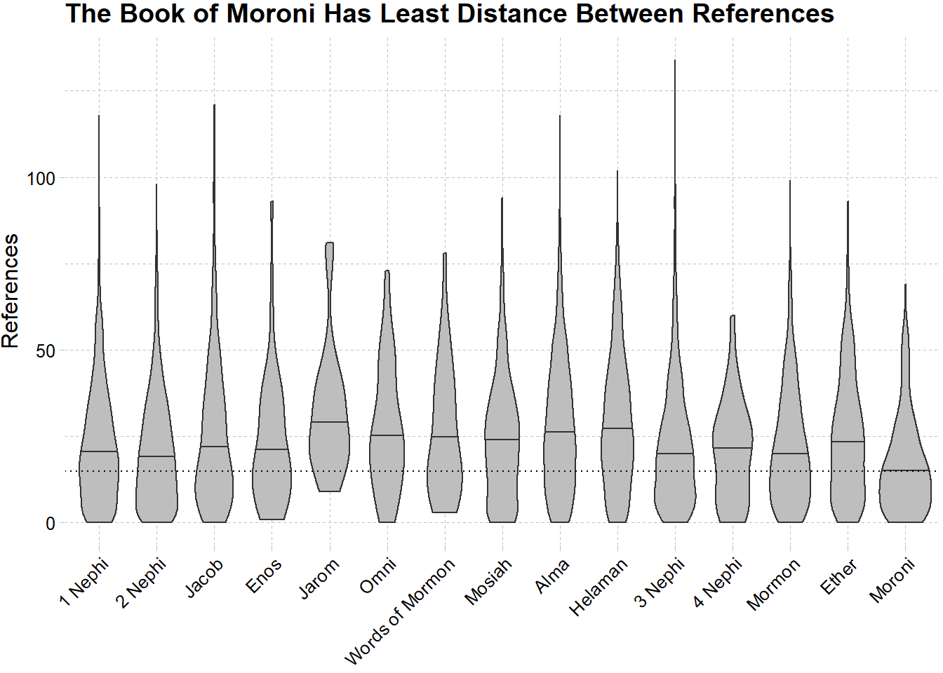
From studying the Book of Mormon, I’m pretty sure the end of Alma and beginning of Helaman is where most of the war chapters are located. What if we wanted to know which book had the least words in between references to Christ?

ggplot(cnt_byverse, aes(x = fct_rev(book_title), y = btw_length)) +
  geom_violin(show.legend = F, fill = "grey", draw_quantiles = c(.5)) +
  #geom_boxplot(col = "black", fill = "grey",width = .3, outlier.shape = NA, show.legend = F) +
  geom_hline(yintercept = 15, linetype = "dotted") +
  labs(x = NULL,
       y = "References",
       title = "The Book of Moroni Has Least Distance Between References") +
  theme_pander() +
  theme(axis.text.x = element_text(angle = 45, vjust = 1,hjust = 1))

Conclusions

We can gather that the war chapters in the Book of Mormon have more content between references of Christ while the book of Moroni has the least on average.