sales <- read_csv("https://byuistats.github.io/M335/data/sales.csv")

Background

Each semester, the business department at BYU-Idaho host the operation for a small number of student organized businesses. They all collected transactional data for us to analyze.

Posing as an investment company, we need to provide a recommendation for the best company to invest in. The decision makers would be better equipped if they know what customer traffic looks like and total income for each of the six companies.

Data Wrangling

• Two rows were removed that were titled “missing.”

• Since transactions for all companies started during the middle of June, a few previous transactions were removed.

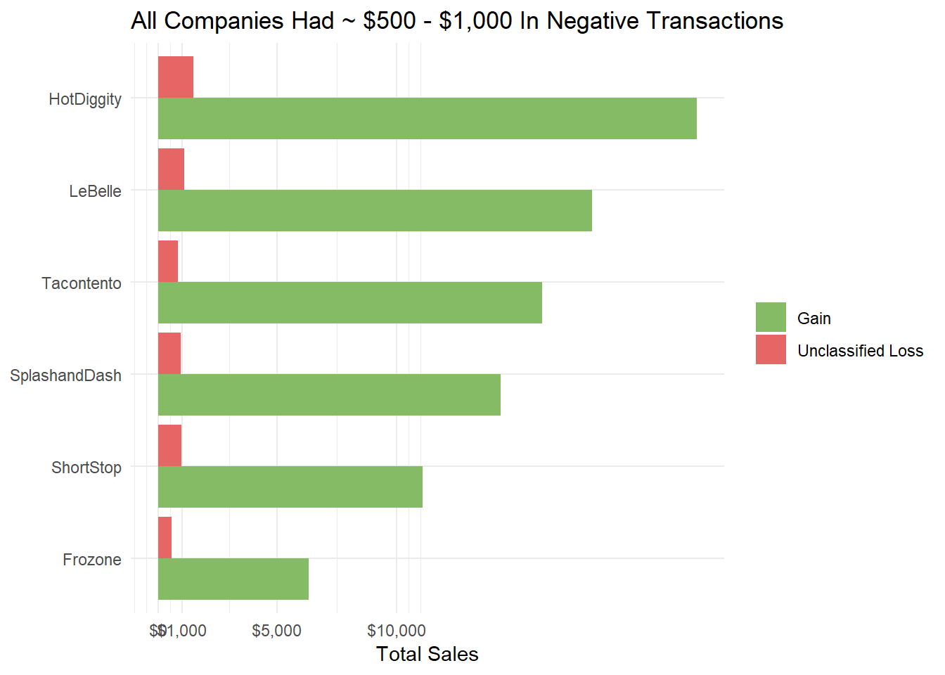
• There were unexplained negative transactions in the amount column, the totals for which is summarized in a plot below.

• Hours, week days, and months were then created from the original date variable.

sales2 <- sales %>% 
  filter(Name != "Missing") %>% 
  mutate(Time = with_tz(Time, "America/Denver"),
         transaction = case_when(
           Amount < 0 ~ "Unclassified Loss",
           Amount >= 0 ~ "Gain"),
         hour = hour(Time),
         hour = factor(hour, levels = c(seq(6,23,1), 0)),
         week_day = wday(Time, label = T),
         month = month(Time))

Data Exploration

As we see below, the data contain negative transactions that aren’t explained. At the time of this analysis, the data collection period occurred two years prior, so we are unable to observe the data generation process. Therefore, I will assume these transactions to be a general loss of total income for each company.

sales2 %>% 
  group_by(Name, transaction) %>%  
  summarise(sum = sum(Amount)) %>%
  mutate(sum = abs(sum)) %>% 
ggplot(aes(fct_reorder(Name, sum, max), y = sum, 
           fill = factor(transaction))) +
  geom_bar(stat = "identity", position = "dodge") +
  scale_y_continuous(labels = scales::dollar,
                     breaks = c(0, 1000, 5000, 10000)) +
  scale_fill_manual(values = c("Unclassified Loss" = "#E66565",
                               "Gain" = "#85bb65")) +
  coord_flip() +
  labs(x = NULL,
       y = "Total Sales",
       fill = NULL,
       title = "All Companies Had ~ $500 - $1,000 In Negative Transactions") +
  theme_minimal()

sales2 %>% 
  filter(Amount > 0) %>% 
ggplot(aes(Name, Amount, fill = Type)) +
  geom_boxplot(outlier.shape = NA) +
  coord_cartesian(ylim = c(0,50)) +
  scale_y_continuous(labels = scales::dollar) +
  scale_fill_few(palette = "Medium") +
  labs(fill = NULL,
       x = NULL,
       y = "Avg. Sale Transaction\n",
       title = "Company Type: Food vs. Goods and Services") +
  theme_minimal()

Customer Traffic

sales2 %>% 
  group_by(Name, week_day, hour) %>% count() %>% 
  filter(week_day != "Sun") %>% 
ggplot(aes(hour, fct_rev(week_day), fill = log(n))) +
  geom_raster() +
  scale_fill_gradient(low = "#DAFADF", high = "#00661D") +
  scale_x_discrete(labels = c(paste0(seq(6,11,1),"AM"), "12PM",
                              paste0(seq(1,11,1),"PM"), "12AM")) +
  facet_grid(Name~.) +
  labs(y = NULL,
       x = NULL,
       fill = "Customer\nTraffic Count",
       title = "Hot Diggity and Tacontento have Highest Customer Traffic",
       subtitle = "Frozone and Tacontento have meaningful Friday evening customer traffic") +
  theme_minimal() +
  theme(strip.text.y = element_text(angle = 0),
        panel.spacing = unit(.75,"lines"))

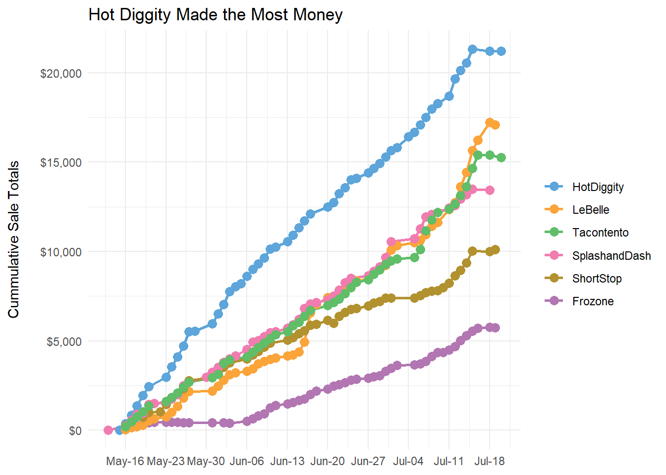
Sales

sales %>% 
  mutate(Time = date(Time)) %>% 
  filter(Time > as.Date("2016-05-01"),
         Name != "Missing") %>% 
  group_by(Name, Time) %>% 
  summarise(sum = sum(Amount)) %>%
  mutate(cm = cumsum(sum)) %>% 
ggplot(aes(Time, cm, 
           col = fct_relevel(Name,
                             c("HotDiggity","LeBelle",
                               "Tacontento","SplashandDash",
                               "ShortStop","Frozone")))) +
  geom_line(size = 1) +
  geom_point(size = 3) +
  scale_color_few(palette = "Medium") +
  scale_y_continuous(labels = scales::dollar) +
  scale_x_date(date_breaks = "1 week",
               date_labels = "%b-%d") +
  labs(col = NULL,
       x = NULL,
       y = "Cummulative Sale Totals\n",
       title = "Hot Diggity Made the Most Money") +
  theme_minimal()

Conclusions

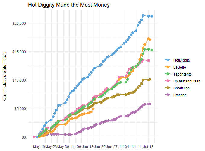
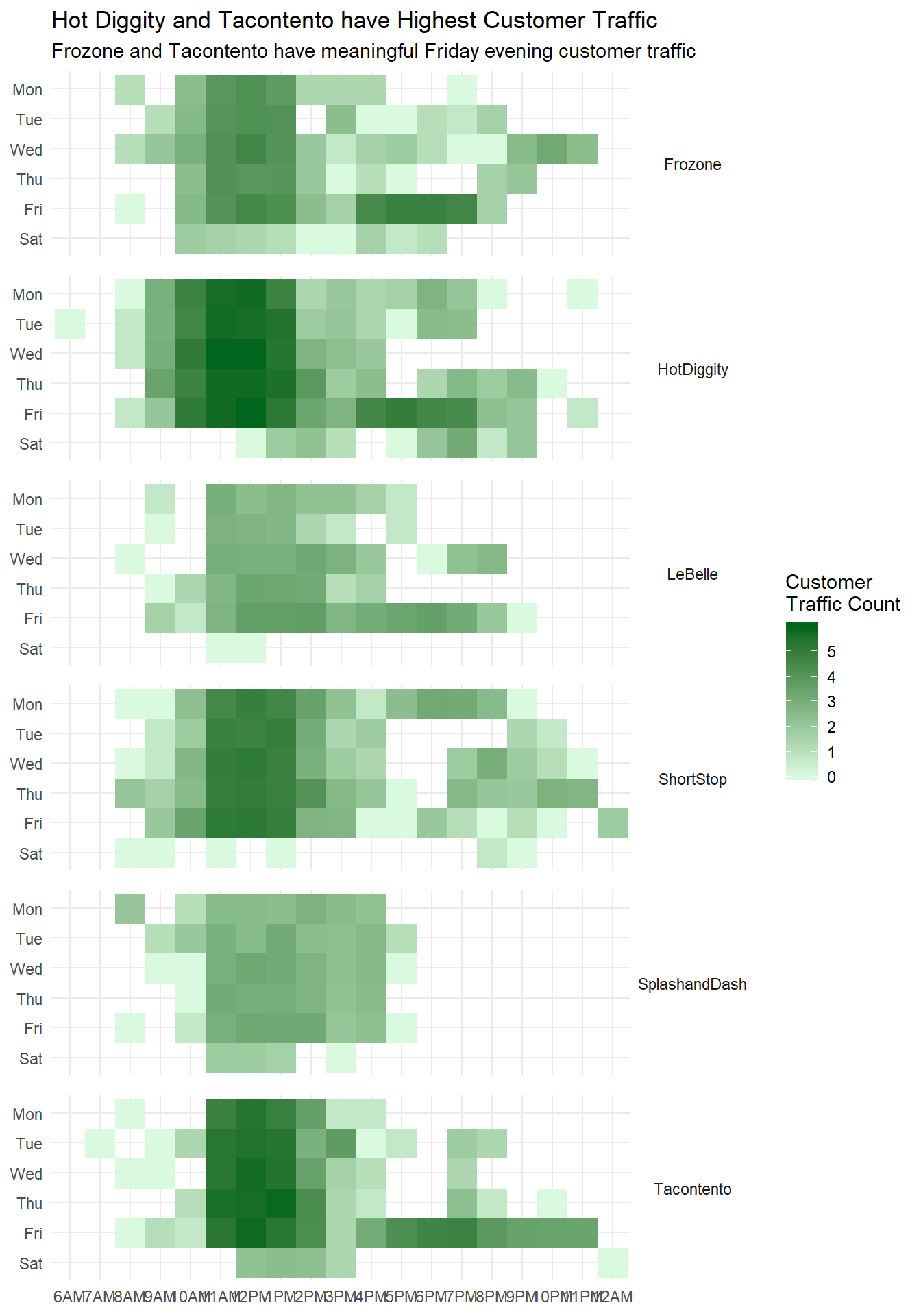
I would recommend investing in Hot Diggity for the following reasons. Hot Diggity maintained consistent increases in sale totals opposed to the competition like LeBelle who seems to have two periods of sporadic increases. This could be due to heavy discounts on their higher priced non-food items and therefore an unrealistic model for long term success. Hot Diggity also has the highest customer traffic. A fluctuation in customer flow would affect Hot Diggity much less than it would LeBelle given LeBelle has a smaller customer base.

Future analysis in encouraged to be conducted during the time of data generation to uncover the reason for negative transactions. We can only speculate now that the occurred due to returns, discounts, or expenses. The occurrence of these negative transactions, as interpreted as a general loss, are shown in the plot above after June 20th when Short Stop saw a significant negative transaction.